Visual representation
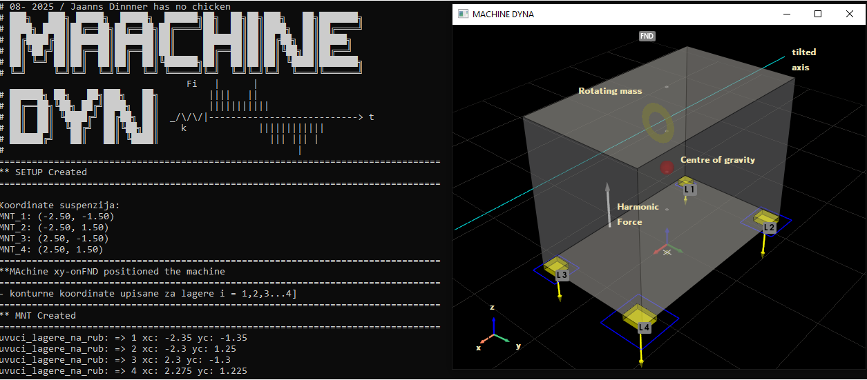
Figure 1: High-level architectural overview of the simulation engine.
Algorithm Architecture & Code Review
Figure 1: High-level architectural overview of the simulation engine.
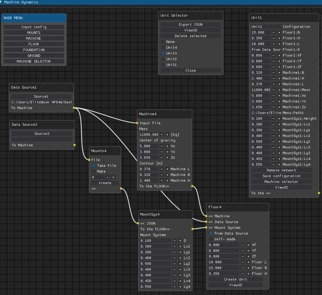
Figure 1: High-level architectural overview of the simulation engine.
This code turned out to be serious piece of engineering work. It isn't just a script; it is a structured 6DOF (Six Degrees of Freedom) Rigid Body Dynamics Simulator utilizing two numerical methods.
_calc, _visual, _solve, _class) enables scalability and isolated testing.Algorithm follows the classic Linear Time-Invariant (LTI) system:
The derivation of stiffness and damping matrices relative to the Center of Gravity (CoG) correctly introduces coupling between translational and rotational motion.
try-except blocks by defining default values instead of duplicating logic.
Future work might be adding non-linear elements (e.g., progressive elastomer stiffness).
ASCII headers and structured comments improve readability and maintain an "engineering-grade" style appreciated in simulation environments.
Prototype turned out to be technically sound, demonstrating strong understanding of both programming and vibration mechanics.
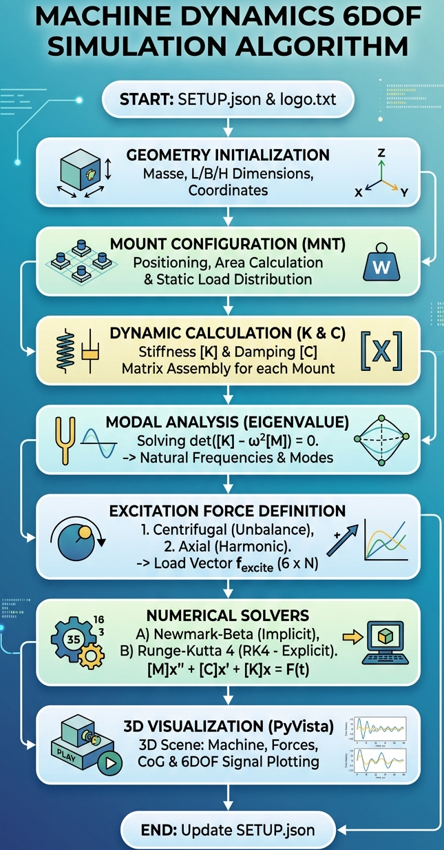
Figure 1: Prototype structure
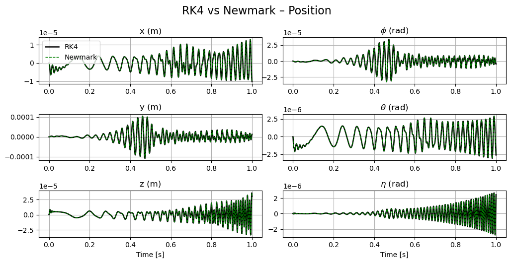
Figure 2: CoG displacements calculated based on forced response of 11.000 tons machine (m),both green and black line, two numeric methods match perfectly for this case.
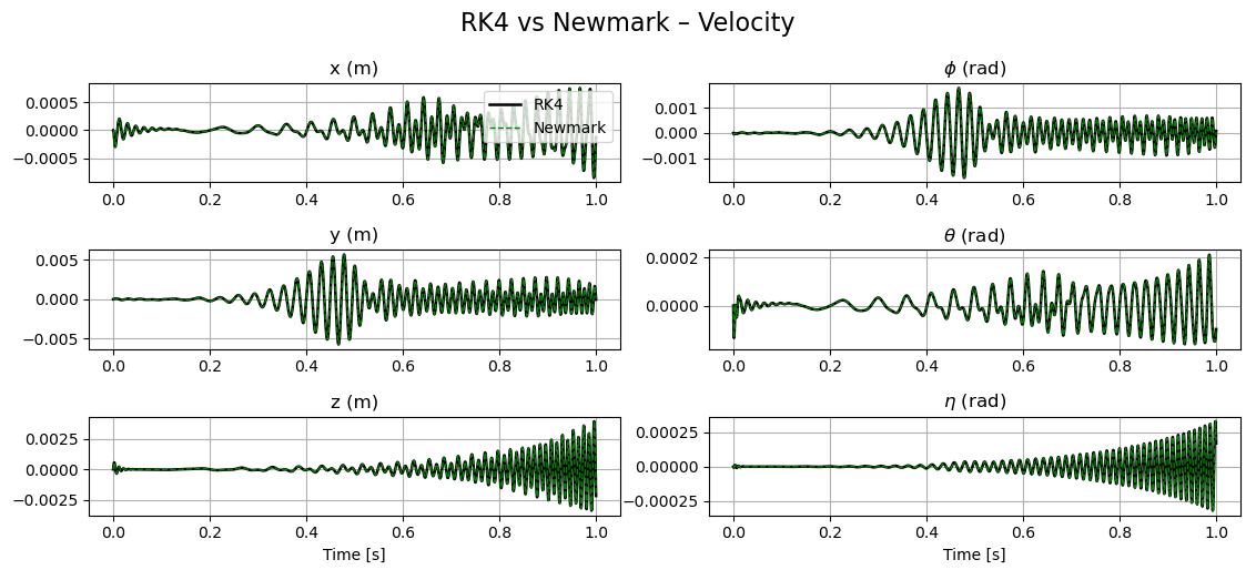
Figure 2: CoG velocities (m/s)
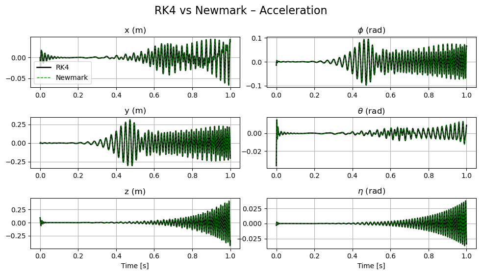
Figure 2: CoG accelerations calculated (m/s2)
	MACH
	├─ Static mass: 11000.0
	├─ Machine_L: 5.0
	├─ Machine_B: 3.0
	├─ Machine_H: 3.65
	├─ Machine_Xs: 0.37
	├─ Machine_Ys: 0.32
	└─ Machine_Zs: 2.4

	DYN
	├─ FORCE_dyn.Fx: 0
	├─ FORCE_dyn.Fy: 0
	├─ FORCE_dyn.Fz: 1000
	├─ X-koordinata: 1.8
	├─ Y-koordinata: 0
	└─ Z-koordinata: 1.5

	FLO
	├─ Floor_L: 10.0
	├─ Floor_B: 15.0
	└─ Floor_H: 0.35

	MNT
	├─ 1: Lx=0.3, Ly=0.3
	├─ 2: Lx=0.4, Ly=0.5
	├─ 3: Lx=0.4, Ly=0.4
	└─ 4: Lx=0.45, Ly=0.55

	calc_MNT
	├─ 1: Lx=0.3, Ly=0.3, AREA_1=0.09, x1=-2.5, y1=-1.5, D=0.15, z1=0.0, xc=-2.35, yc=-1.35
	├─ 2: Lx=0.4, Ly=0.5, AREA_2=0.2, x2=-2.5, y2=1.5, D=0.15, z2=0.0, xc=-2.3, yc=1.25
	├─ 3: Lx=0.4, Ly=0.4, AREA_3=0.16, x3=2.5, y3=-1.5, D=0.15, z3=0.0, xc=2.3, yc=-1.3
	└─ 4: Lx=0.45, Ly=0.55, AREA_4=0.2475, x4=2.5, y4=1.5, D=0.15, z4=0.0, xc=2.275, yc=1.225

	calc_STATIC
	├─ m_tot[kg]: 11000.0
	├─ A_tot[m2]: 0.698
	├─ s_tot[N/mm2]: 0.155
	├─ s_tot[N/m2]: 154709.677
	├─ Fs_tot[N]: 107910.0
	├─ Fs_tot->[kN]: 107.91
	├─ L1 [kN]: 13.924
	├─ L2 [kN]: 30.942
	├─ L3 [kN]: 24.754
	└─ L4 [kN]: 38.291

	calc_DYN
	├─ fx[Hz]: 16
	├─ fy[Hz]: 16
	├─ fz[Hz]: 21
	├─ zeta_X: 0.1
	├─ zeta_Y: 0.1
	├─ zeta_Z: 0.15
	├─ K1: kx1=14344674.022, ky1=14344674.022, kz1=24710942.359
	├─ K2: kx2=31877053.383, ky2=31877053.383, kz2=54913205.241
	├─ K3: kx3=25501642.706, ky3=25501642.706, kz3=43930564.193
	├─ K4: kx4=39447853.561, ky4=39447853.561, kz4=67955091.486
	├─ C1: cx1=28537.822, cy1=28537.822, cz1=56183.837
	├─ C2: cx2=63417.383, cy2=63417.383, cz2=124852.972
	├─ C3: cx3=50733.906, cy3=50733.906, cz3=99882.378
	└─ C4: cx4=78479.011, cy4=78479.011, cz4=154505.553

	calc_EXCITE
	├─ t_start: 0
	├─ t_finish: 5
	├─ iteracija: 4096
	├─ fs: 819.2
	├─ Centrifugal Force: True
	├─ f_start: 1
	├─ f_finish: 10
	├─ C: x=0.0, y=0.0, z=3.1025
	├─ m_c: 2.0
	├─ r_c: 0.25
	├─ rot_axis: [1.0, 0.0, 0.0]
	├─ e1: [0.0, -1.0, 0.0]
	├─ e2: [0.0, 0.0, -1.0]
	├─ Aksijalne sile: True
	├─ fo: 0
	├─ fend: 5
	├─ Aksijalna sila: True
	├─ Fx: 0
	├─ Fy: 0
	├─ Fz: 1000
	├─ magnituda: 1000.0
	├─ jedinicni: [0.0, 0.0, 1.0]
	└─ K: x=1.8, y=0, z=1.5

	calc_MODAL
	├─ 1: frequency=8.114, active_dofs=y, θx
	├─ 2: frequency=11.798, active_dofs=x
	├─ 3: frequency=21.0, active_dofs=z
	├─ 4: frequency=23.456, active_dofs=θz
	├─ 5: frequency=33.055, active_dofs=x, y, θx, θy
	└─ 6: frequency=34.492, active_dofs=x, y, θx, θy